An Isoform resoloution single cell RNA-seq toolkit.
Allos_logo
Single-cell RNA sequencing (scRNA-seq) has revolutionized our understanding of cellular diversity by allowing the study of gene expression at the individual cell level. However, traditional methods of quantification obscure the most fine-grained transcriptional layer—the individual transcripts at sequence-level resolution—in favor of gene-level binning. This strategy is useful when the sequencing read length is short, as it avoids the difficult task of transcript assembly, which is made even more challenging by the nature of single-cell data.
Traditional scRNA-seq methods often rely on short-read sequencing technologies, which can limit the ability to resolve full-length transcripts and isoforms. Long-read sequencing technologies, such as those provided by Oxford Nanopore and PacBio, overcome this limitation by producing reads that span entire transcripts. This capability is crucial for accurately identifying and characterizing novel isoforms and understanding the complexity of transcriptomes in single cells. By integrating long-read sequencing with single-cell approaches, researchers can gain deeper insights into cellular heterogeneity and the functional implications of transcriptomic variations.
Allos is designed to give users familiar with single-cell analysis, and indeed object-oriented programming in general, an extended toolkit wrapping around Scanpy and the wider scverse to facilitate analysis workflows of this type of data. Allos is the culmination of many smaller individualized scripts packaged together into a common framework centered on anndata objects. It also contains many recreations (of varying faithfulness to their originals*) of functions proposed by others in other libraries, languages, or contexts—we by no means intend to plagiarize these methods but only expand them to a wider audience.
Allos intends to offer a full suite of modules for every step of single-cell isoform resolution data, from preprocessing, working with annotations, plotting, identifying differential features, isoform switches, and more. We hope to expand Allos with the input of our user base as the field of long-read single-cell further matures.
Install
pip install allos
Basic workflow
The first thing we need to work with Allos is data. Our goal is for Allos to handle many, if not all, types of single-cell isoform resolution data, making it platform and protocol agnostic. While it is important to consider the biases, strengths, limitations, and caveats of each approach, all methods utilize a transcript matrix from which a gene matrix can be derived. Allos also allows users to supply their own custom annotations in the form of a GTF or use a reference annotation. If a reference annotation is provided, all plotting functions will use the underlying GTF to retrieve the transcript information.
To help you follow the basic workflow, we provide an easy way to download one of our test datasets. The Sicelore dataset comprises 1,121 single-cell transcriptomes from two technical replicates derived from an embryonic day 18 (E18) mouse brain, consisting of 951 cells and 190 cells. The dataset was generated using the 10x Genomics Chromium system and sequenced with both Oxford Nanopore and Illumina platforms, producing 322 million Nanopore reads and 70 million Illumina reads for the 951-cell replicate, and 32 million Nanopore reads with 43 million Illumina reads for the 190-cell replicate. The dataset captured a median of 2,427 genes and 6,047 UMIs per cell, enabling the identification of 33,002 annotated transcript isoforms and 4,388 novel isoforms. Major cell types in the dataset include radial glia, cycling radial glia, intermediate progenitors, Cajal-Retzius cells, and maturing GABAergic and glutamatergic neurons, providing a detailed resource for studying transcriptome-wide alternative splicing, isoform expression, and sequence diversity during mouse brain development.
import allos.preprocessing as ppsicelore_mouse_data = pp.process_mouse_data()
🔎 Looking for file at: /data/analysis/data_mcandrew/Allos_new/allos_env/lib/python3.10/site-packages/allos/resources/e18.mouse.clusters.csv
✅ File found at: /data/analysis/data_mcandrew/Allos_new/allos_env/lib/python3.10/site-packages/allos/resources/e18.mouse.clusters.csv
✅ File already exists at: /data/analysis/data_mcandrew/Allos_new/allos_env/lib/python3.10/site-packages/allos/resources/data/mouse_1.txt.gz

🔄 Decompressing /data/analysis/data_mcandrew/Allos_new/allos_env/lib/python3.10/site-packages/allos/resources/data/mouse_1.txt.gz to /data/analysis/data_mcandrew/Allos_new/allos_env/lib/python3.10/site-packages/allos/resources/data/mouse_1.txt...
✅ Decompression complete.
Test data (mouse_1) downloaded successfully
✅ File already exists at: /data/analysis/data_mcandrew/Allos_new/allos_env/lib/python3.10/site-packages/allos/resources/data/mouse_2.txt.gz

🔄 Decompressing /data/analysis/data_mcandrew/Allos_new/allos_env/lib/python3.10/site-packages/allos/resources/data/mouse_2.txt.gz to /data/analysis/data_mcandrew/Allos_new/allos_env/lib/python3.10/site-packages/allos/resources/data/mouse_2.txt...
✅ Decompression complete.
Test data (mouse_2) downloaded successfully
/data/analysis/data_mcandrew/Allos_new/allos_env/lib/python3.10/site-packages/anndata/_core/anndata.py:1756: UserWarning: Observation names are not unique. To make them unique, call `.obs_names_make_unique`.
  utils.warn_names_duplicates("obs")
In this dataset, we observe the mouse data organized in a cell-by-transcript matrix format. This structure allows us to examine the expression levels of individual transcripts across different cells. Additionally, each transcript is associated with a specific gene, providing a hierarchical view of gene expression. This organization is crucial for understanding the relationship between transcripts and their corresponding genes.
sicelore_mouse_data
View of AnnData object with n_obs × n_vars = 1109 × 31986
    obs: 'batch', 'cell_type'
    var: 'geneId'
Lets take a look at our data. An AnnData object is a core data structure used in Scanpy to store single-cell data, including gene or isoform expression counts. It organizes the expression matrix alongside rich metadata: cell-level annotations (.obs), feature-level annotations (.var), and optional layers like normalized data, embeddings (.obsm), and graphs (.obsp). It supports both in-memory and on-disk (HDF5-backed) storage, making it efficient for large-scale single-cell transcriptomics datasets.
IsoAdata objects are fully compatible with standard AnnData objects. We can use them just like any conventional AnnData instance. Let’s take a closer look at how they function.
The .var of an anndata object is a Pandas dataframe. Pandas is a Python library for data manipulation and analysis, built around two core structures: DataFrame (2D tables) and Series (1D arrays). It provides fast, intuitive tools for filtering, transforming, summarizing, and joining structured data. This makes it really easy to preform any manipulations we may need. Lets get our .var in a more usable format.
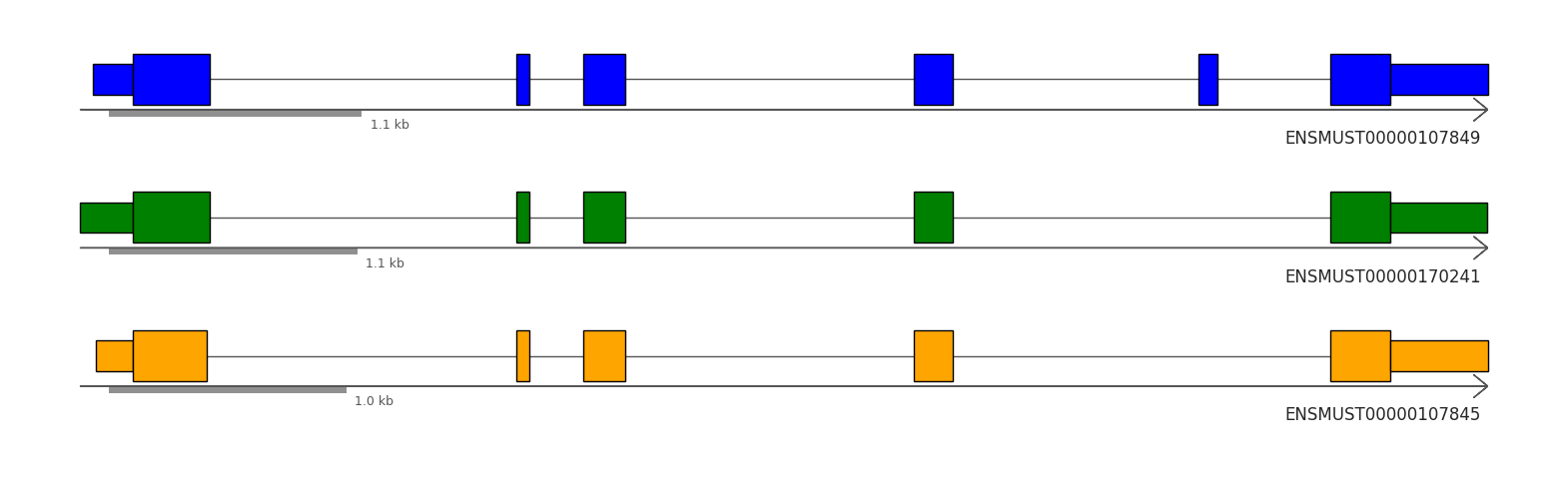
Lets take a quick look at an individual gene CLTA and examine some of its transcripts.
# sanity checkprint("\nAll CLTA isoforms still present:")display(sicelore_mouse_data.var.query("geneId == 'Clta'").head())
All CLTA isoforms still present:
geneId
transcriptId
ENSMUST00000107851.9
Clta
ENSMUST00000107845.3
Clta
ENSMUST00000107846.9
Clta
ENSMUST00000170241.7
Clta
ENSMUST00000107849.9
Clta
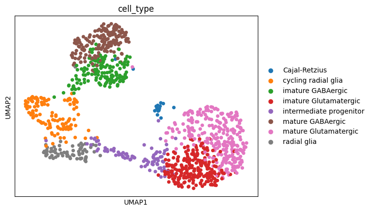
import scanpy as sc# Make a copy of the original data to preserve itoriginal_sicelore_mouse_data = sicelore_mouse_data.copy()# Perform the operationssc.pp.normalize_total(sicelore_mouse_data, target_sum=1e6)sc.pp.log1p(sicelore_mouse_data)# Select the top 5000 highly variable genessc.pp.highly_variable_genes(sicelore_mouse_data, n_top_genes=5000)sicelore_mouse_data = sicelore_mouse_data[:, sicelore_mouse_data.var.highly_variable]sc.pp.neighbors(sicelore_mouse_data)sc.tl.umap(sicelore_mouse_data)sc.pl.umap(sicelore_mouse_data, color='cell_type')# Restore the original datasicelore_mouse_data = original_sicelore_mouse_data
/home/mcandrew/.local/lib/python3.10/site-packages/scanpy/preprocessing/_normalization.py:207: UserWarning: Received a view of an AnnData. Making a copy.
  view_to_actual(adata)
/home/mcandrew/.local/lib/python3.10/site-packages/scanpy/tools/_utils.py:41: UserWarning: You’re trying to run this on 5000 dimensions of `.X`, if you really want this, set `use_rep='X'`.
         Falling back to preprocessing with `sc.pp.pca` and default params.
  warnings.warn(
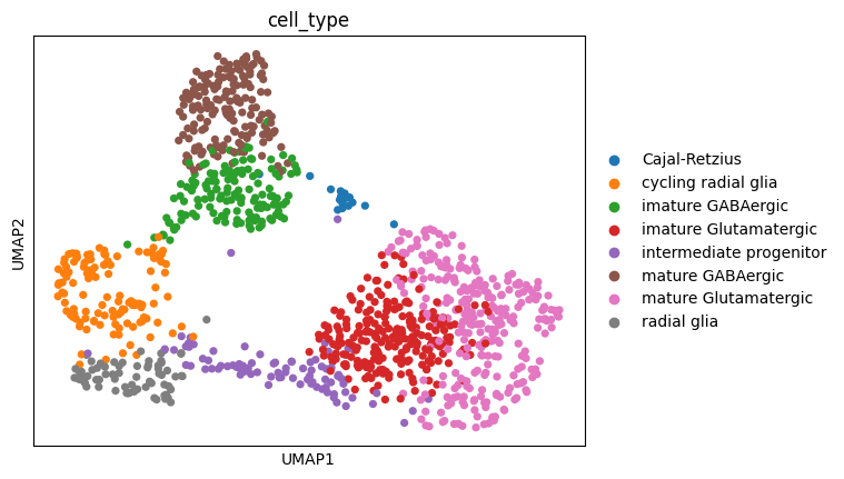
We can easily collapse the transcript matrix to a gene matrix and see how the dimensionality reduction plot differs.
import allos.preprocessing as ppgene_anndata = pp.get_sot_gene_matrix(sicelore_mouse_data)# Make a copy of the gene matrix data to preserve itoriginal_gene_anndata = gene_anndata.copy()# Perform the operations on the gene matrixsc.pp.normalize_total(gene_anndata, target_sum=1e6)sc.pp.log1p(gene_anndata)# Select the top 5000 highly variable genes for gene_anndatasc.pp.highly_variable_genes(gene_anndata, n_top_genes=2000)gene_anndata = gene_anndata[:, gene_anndata.var.highly_variable]sc.pp.neighbors(gene_anndata)sc.tl.umap(gene_anndata)sc.pl.umap(gene_anndata, color='cell_type')# Restore the original gene matrix datagene_anndata = original_gene_anndata
/home/mcandrew/.local/lib/python3.10/site-packages/scanpy/tools/_utils.py:41: UserWarning: You’re trying to run this on 2014 dimensions of `.X`, if you really want this, set `use_rep='X'`.
         Falling back to preprocessing with `sc.pp.pca` and default params.
  warnings.warn(
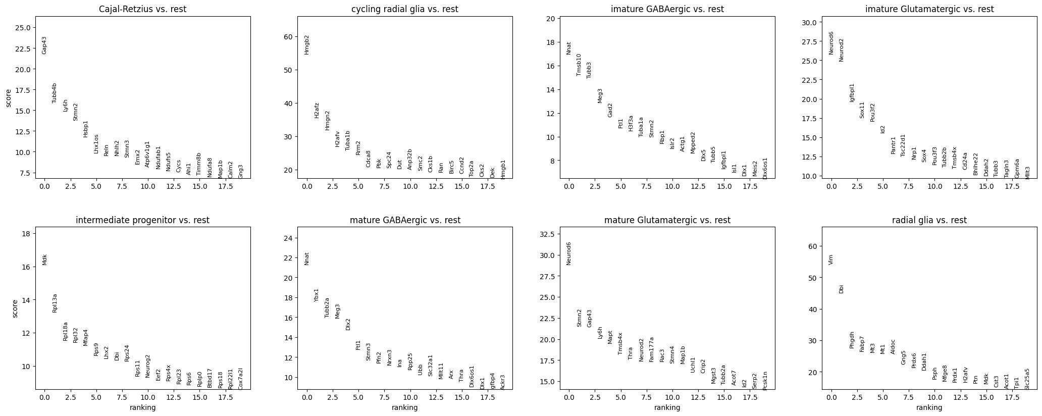
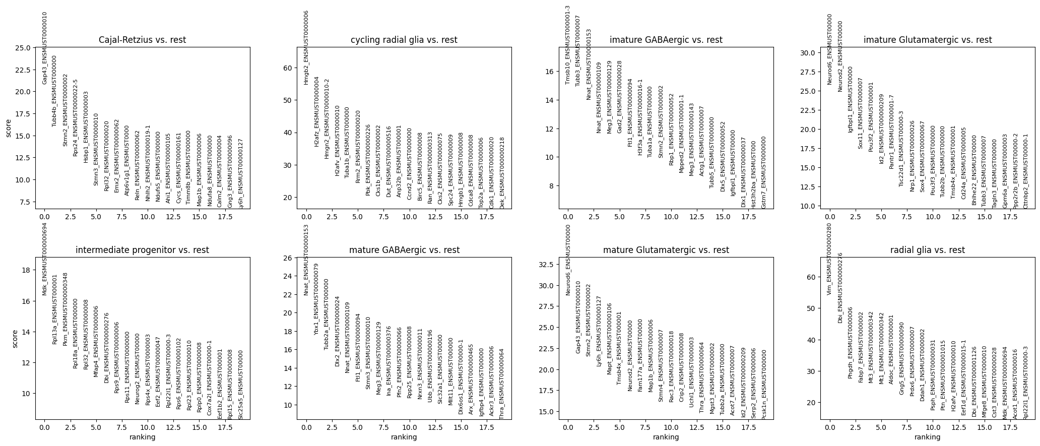
Let’s examine the most differentially expressed genes across the pre-annotated cell types.
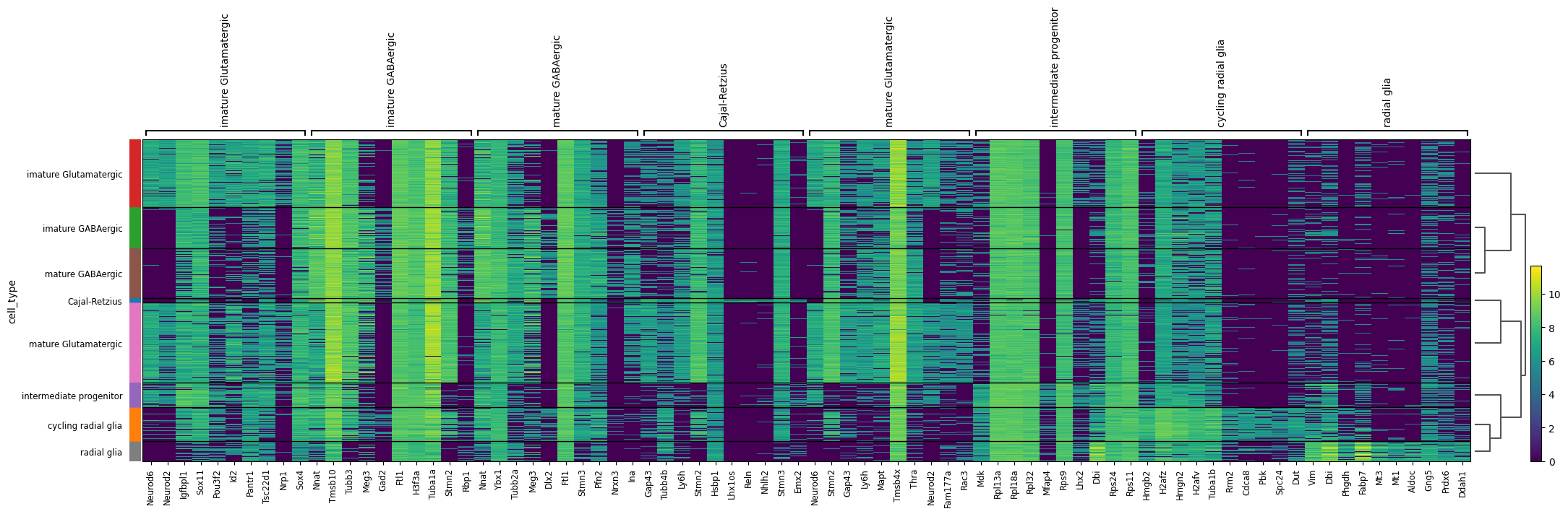
sc.pp.normalize_total(gene_anndata, target_sum=1e6)sc.pp.log1p(gene_anndata)# Perform differential expression analysis to rank genes on the gene matrixsc.tl.rank_genes_groups(gene_anndata, 'cell_type', method='t-test')# Plot the ranked gene groups with adjusted figure sizesc.pl.rank_genes_groups(gene_anndata, n_genes=20, sharey=False, figsize=(12, 10))sc.pl.rank_genes_groups_heatmap(gene_anndata, show_gene_labels=True)
WARNING: dendrogram data not found (using key=dendrogram_cell_type). Running `sc.tl.dendrogram` with default parameters. For fine tuning it is recommended to run `sc.tl.dendrogram` independently.
/home/mcandrew/.local/lib/python3.10/site-packages/scanpy/tools/_utils.py:41: UserWarning: You’re trying to run this on 12561 dimensions of `.X`, if you really want this, set `use_rep='X'`.
         Falling back to preprocessing with `sc.pp.pca` and default params.
  warnings.warn(
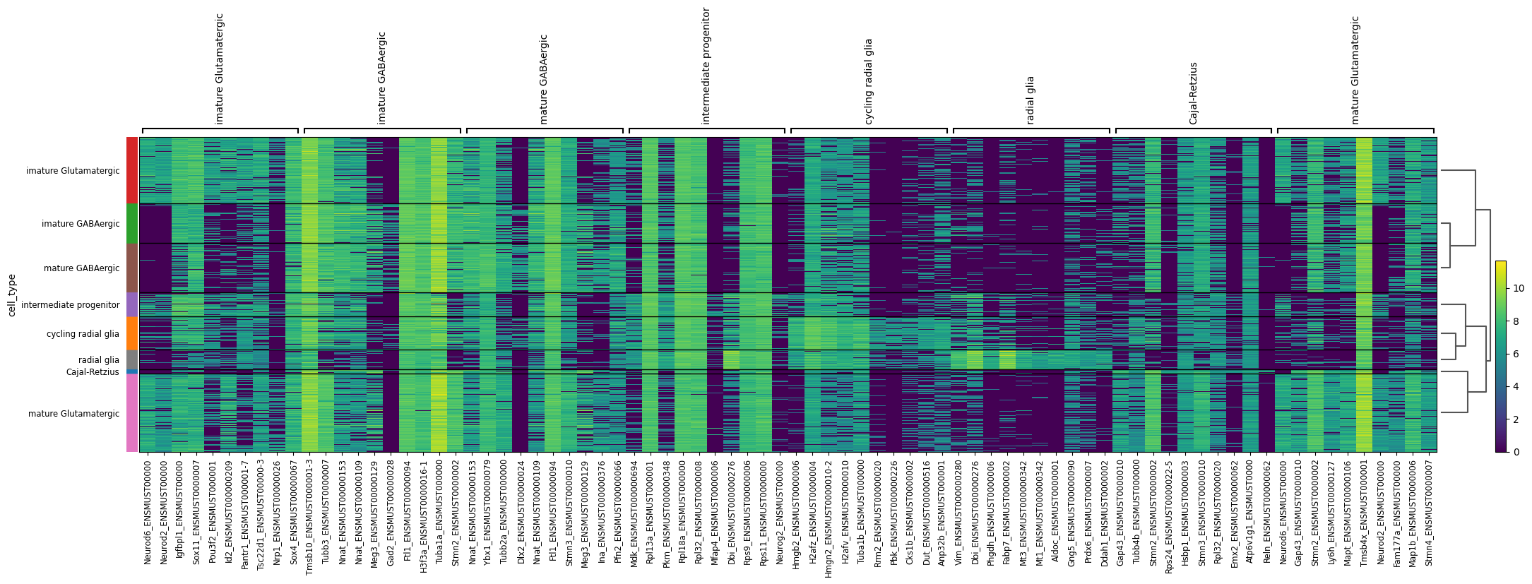
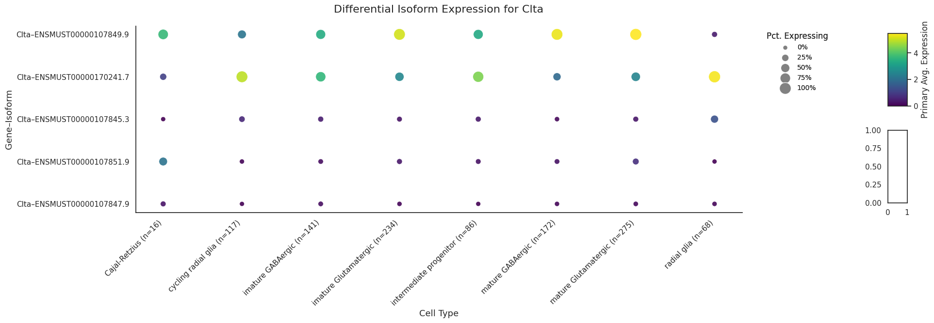
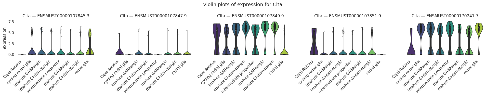
Now, let’s examine the differentially expressed transcripts. Unlike our previous focus on genes, we will shift our attention to the transcript level. The finest resoloution transcriptional layer. We should still see considerable gene wise overlap in the two rankings as we would expect in many cases the higher gene count to be driven by a single isoform.
# Concatenate the gene name before the transcript ID in the transcript matrixtranscript_matrix = sicelore_mouse_data.copy()# Convert 'geneId' to string to avoid TypeError when concatenating with indextranscript_matrix.var['geneId'] = transcript_matrix.var['geneId'].astype(str)# Assuming 'gene_name' and 'transcript_id' are columns in the var DataFrame of the AnnData objecttranscript_matrix.var['gene_transcript_id'] = transcript_matrix.var['geneId'] +'_'+ transcript_matrix.var.index.astype(str)# Truncate the gene_transcript_id to fit better in plotstranscript_matrix.var['gene_transcript_id'] = transcript_matrix.var['gene_transcript_id'].str.slice(0, 20)# Update the var index to use the new truncated gene_transcript_idtranscript_matrix.var.index = transcript_matrix.var['gene_transcript_id']transcript_matrix.var_names_make_unique()# Log transform and CPM normalize the transcript matrixsc.pp.normalize_total(transcript_matrix, target_sum=1e6)sc.pp.log1p(transcript_matrix)# Perform differential expression analysis to rank genes on the transcript matrixsc.tl.rank_genes_groups(transcript_matrix, 'cell_type', method='t-test')# Plot the ranked gene groups with adjusted figure sizesc.pl.rank_genes_groups(transcript_matrix, n_genes=20, sharey=False, figsize=(12, 10))sc.pl.rank_genes_groups_heatmap(transcript_matrix, show_gene_labels=True)
WARNING: dendrogram data not found (using key=dendrogram_cell_type). Running `sc.tl.dendrogram` with default parameters. For fine tuning it is recommended to run `sc.tl.dendrogram` independently.
/home/mcandrew/.local/lib/python3.10/site-packages/scanpy/tools/_utils.py:41: UserWarning: You’re trying to run this on 31986 dimensions of `.X`, if you really want this, set `use_rep='X'`.
         Falling back to preprocessing with `sc.pp.pca` and default params.
  warnings.warn(
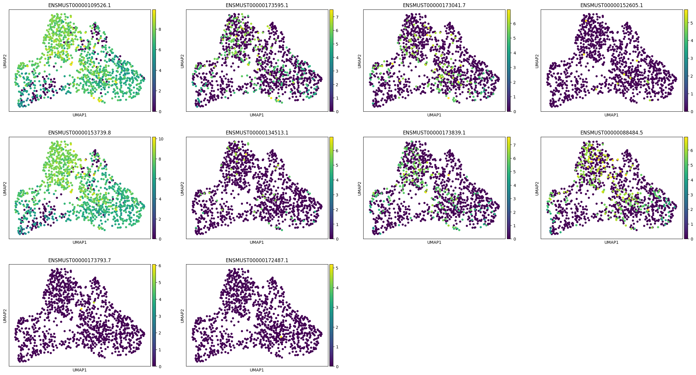
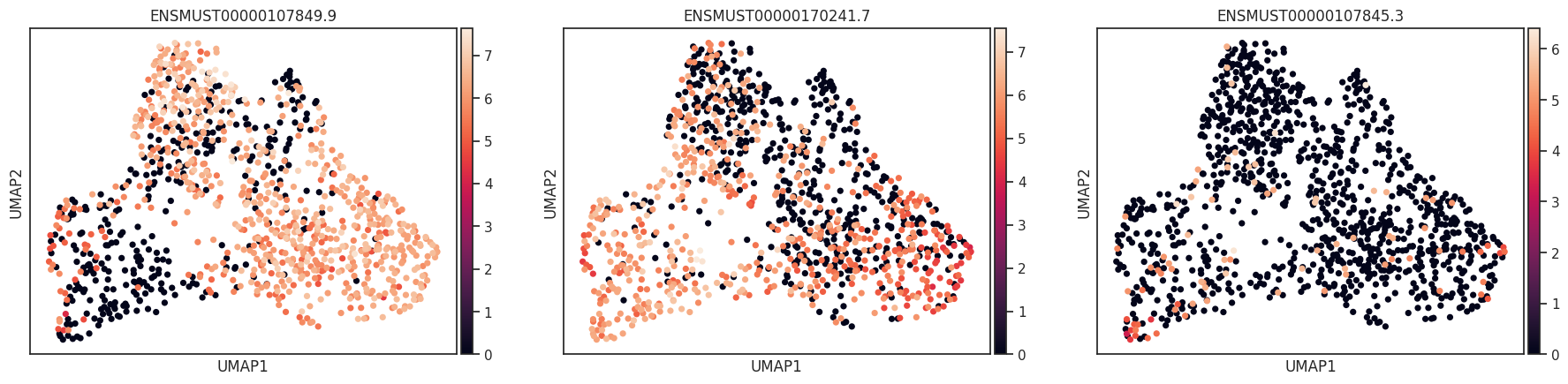
Lets visualise the isoforms of a specific gene Nnat based on multiple transcripts from this gene in the top rankings of imature GABAergic vs rest.
# Perform the operations on a copy of the sicelore_mouse_datasicelore_mouse_data_copy = sicelore_mouse_data.copy()sc.pp.normalize_total(sicelore_mouse_data_copy, target_sum=1e6)sc.pp.log1p(sicelore_mouse_data_copy)sc.pp.neighbors(sicelore_mouse_data_copy)sc.tl.umap(sicelore_mouse_data_copy)
/home/mcandrew/.local/lib/python3.10/site-packages/scanpy/tools/_utils.py:41: UserWarning: You’re trying to run this on 31986 dimensions of `.X`, if you really want this, set `use_rep='X'`.
         Falling back to preprocessing with `sc.pp.pca` and default params.
  warnings.warn(
import allos.visuals as vsvs.plot_transcripts(sicelore_mouse_data_copy, gene_id='Nnat')
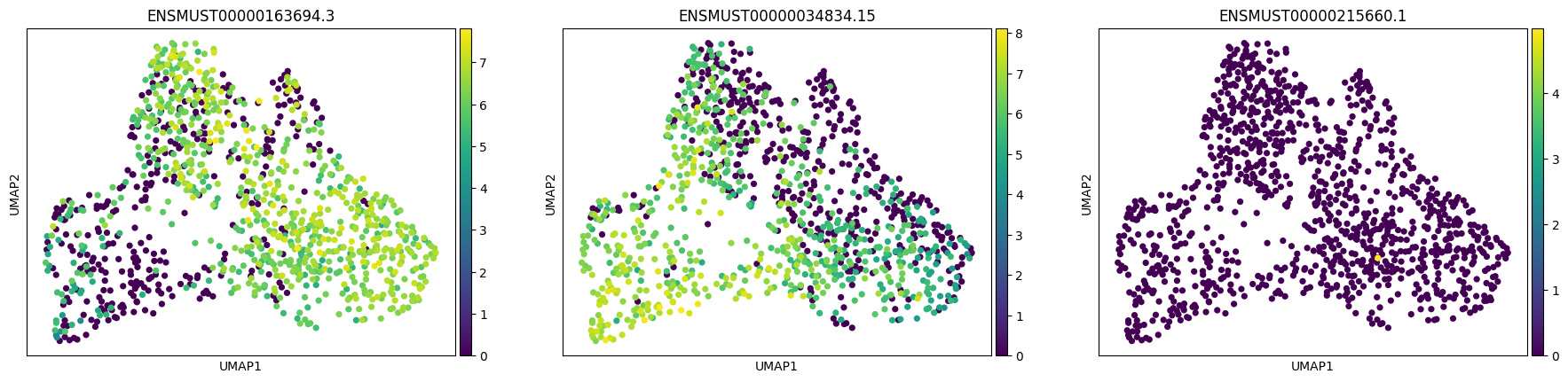
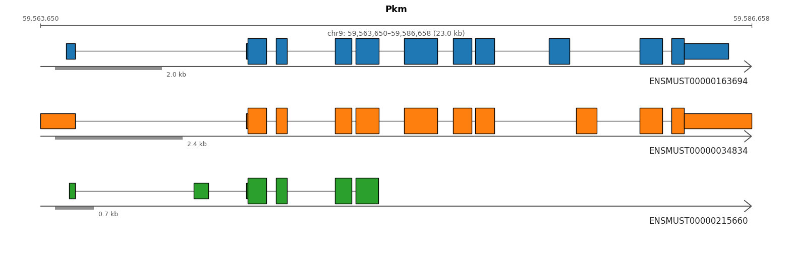
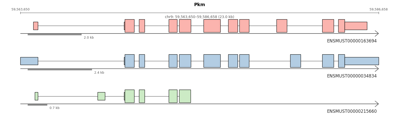
import allos.visuals as vsvs.plot_transcripts(sicelore_mouse_data_copy, gene_id='Pkm')
/data/analysis/data_mcandrew/Allos_new/allos_env/lib/python3.10/site-packages/allos/visuals.py:474: UserWarning: set_ticklabels() should only be used with a fixed number of ticks, i.e. after set_ticks() or using a FixedLocator.
  ax.set_xticklabels(new_labels, rotation=45, ha='right', fontsize=11)
/data/analysis/data_mcandrew/Allos_new/allos_env/lib/python3.10/site-packages/allos/visuals.py:474: UserWarning: set_ticklabels() should only be used with a fixed number of ticks, i.e. after set_ticks() or using a FixedLocator.
  ax.set_xticklabels(new_labels, rotation=45, ha='right', fontsize=11)
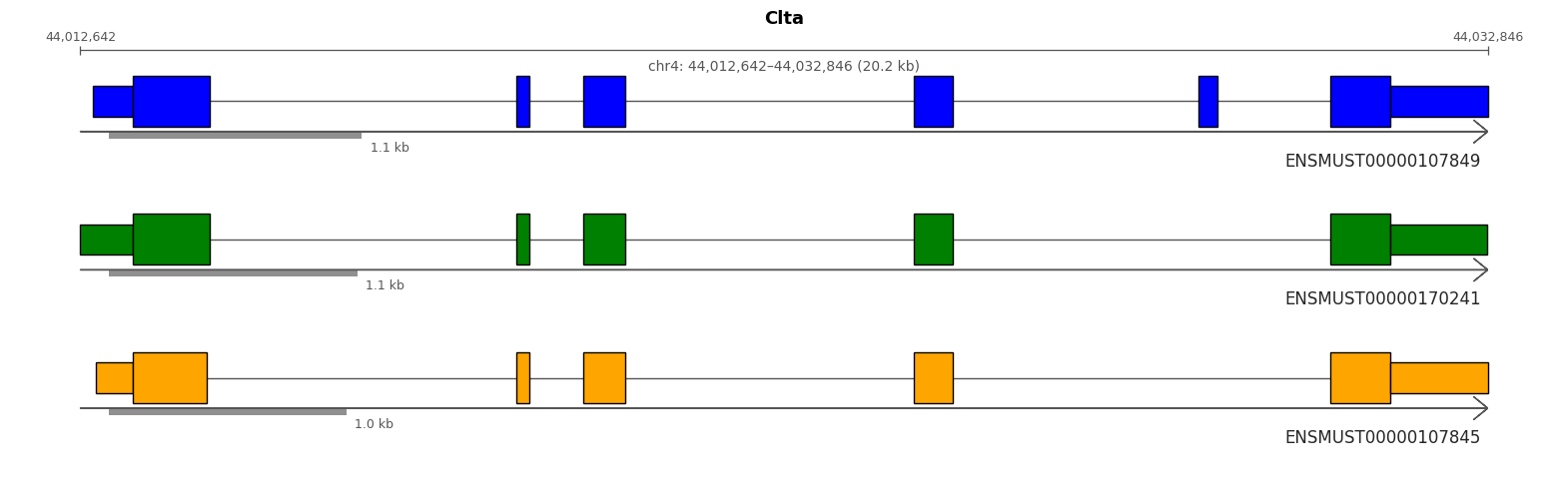
Let’s explore these transcripts of interest by visualizing them using the method described below. We will instantiate our transcript plot objects with the appropriate GTF file. For demonstration purposes, we provide the code to download the GTF file used in this dataset. This process will help us better understand the structure of the transcripts involved in this Isoform switch. Please ensure that you have a stable internet connection to download the GTF file if it’s not already available locally.
from allos.transcript_plots import TranscriptPlotsimport osimport urllib.requestfrom pathlib import Path# Example Ensembl URLs for mouse GRCm39 (release 109)gtf_url ="ftp://ftp.ensembl.org/pub/release-109/gtf/mus_musculus/Mus_musculus.GRCm39.109.gtf.gz"# Store data one directory backdata_dir = Path("..") /"data"data_dir.mkdir(parents=True, exist_ok=True)gtf_file_local = data_dir /"Mus_musculus.GRCm39.109.gtf.gz"# Download if not already presentifnot gtf_file_local.is_file():print(f"Downloading {gtf_url}...") urllib.request.urlretrieve(gtf_url, gtf_file_local)
from allos.transcript_data import TranscriptData# Instantiate your TranscriptDatatd = TranscriptData( gtf_file=gtf_file_local)
from allos.transcript_plots import TranscriptPlots
from allos.switch_search import get_top_n_isoforms
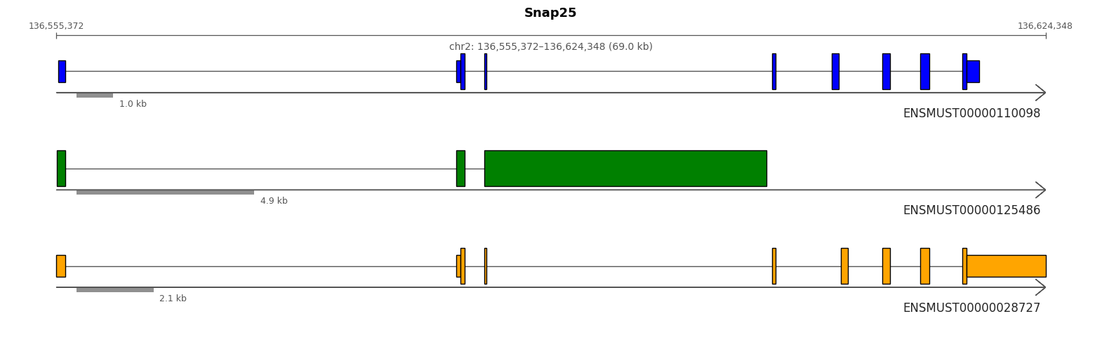
from allos.switch_search import get_top_n_isoformstop_n = get_top_n_isoforms(sicelore_mouse_data_copy, gene_id='Snap25', strip=True)tp.draw_transcripts_list(top_n, draw_cds=True, show_ticks=True)
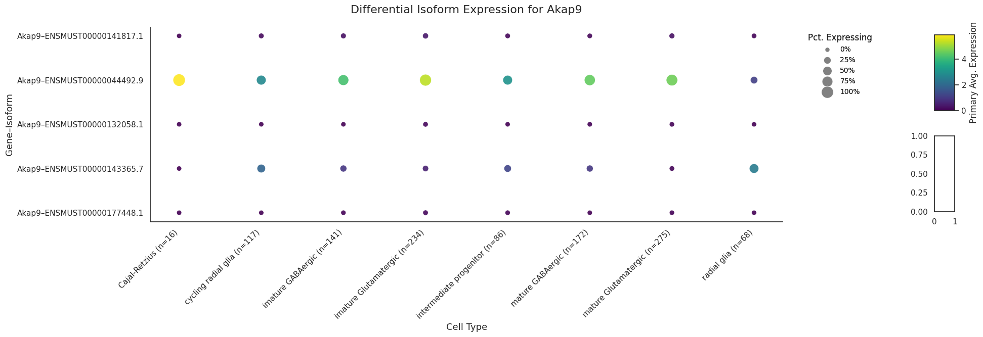
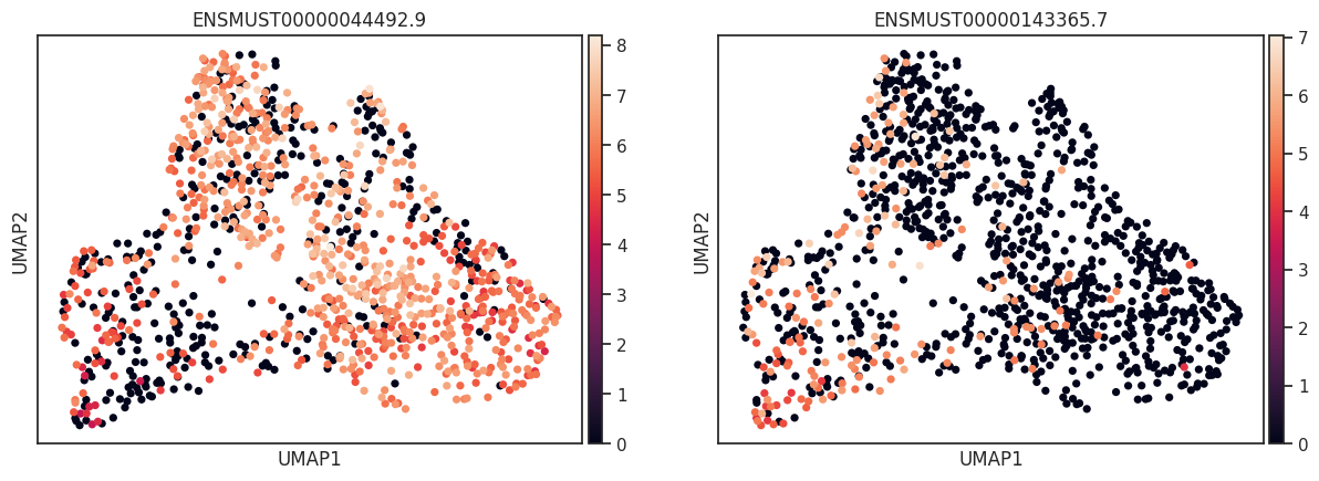
To focus on the top three most expressed isoforms in the dataset, we can filter and visualize them using the following approach. This allows us to concentrate on the most significant isoforms for further analysis or presentation, useful as some genes have a lot of isoforms and many are very lowly exspressed.
To gain a deeper understanding of how isoforms structurally differ across various cell types, we can analyze the inclusion of different exons in the final transcript structure. A useful metric for this analysis is the Percent Spliced In (PSI) value, which quantifies the proportion of transcripts that include a particular exon. By calculating the PSI for each exon, we can identify and compare the structural variations of isoforms between cell types, providing insights into their functional implications and regulatory mechanisms. This approach allows us to pinpoint specific exons that contribute to the diversity of isoform expression and understand their role in cellular differentiation and function.
Let’s explore another potential isoform switch event.
/data/analysis/data_mcandrew/Allos_new/allos_env/lib/python3.10/site-packages/allos/visuals.py:474: UserWarning: set_ticklabels() should only be used with a fixed number of ticks, i.e. after set_ticks() or using a FixedLocator.
  ax.set_xticklabels(new_labels, rotation=45, ha='right', fontsize=11)
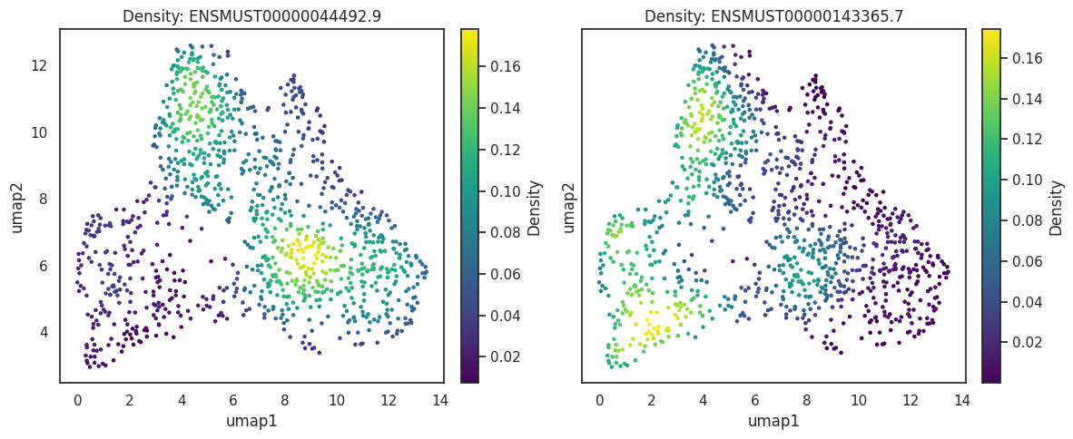
The visualization of cell features, such as genes and peaks, is often challenged by sparsity and technical dropout. These factors can obscure the clarity of visualizations, particularly when combined with clustering techniques used to annotate cell types. To enhance the visibility of patterns within the data, kernel density estimation (KDE) can be employed. KDE helps to highlight underlying trends by smoothing the data, making patterns more pronounced. However, it is crucial to use KDE alongside the actual count data to avoid potential misinterpretations. Relying solely on KDE without considering the raw counts can lead to misleading conclusions, as it may exaggerate or obscure the true distribution of features. Therefore, a balanced approach that integrates both KDE and raw data visualization is recommended for accurate interpretation.